“Good work!”
— Abhishek, 12/13/2019
“It’s a bad model”
— Abhishek, 12/16/2019
For last week’s project at the Flatiron School, my partner Dayana and I investigated the effect of bad weather on transportation patterns in Chicago. We used hourly weather data to create a dummy variable to represent “bad weather” on a given day, and then tested our null hypothesis that daily CTA ridership during bad weather is the same as CTA ridership during good weather.
Lo and behold, the p-value was less than 0.01:
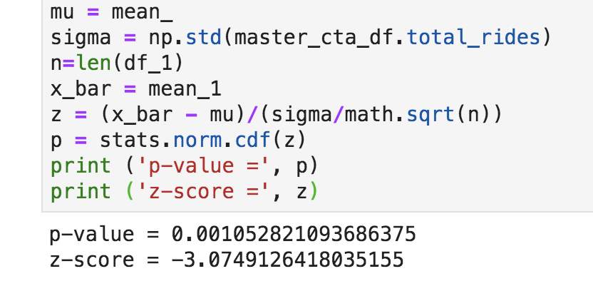
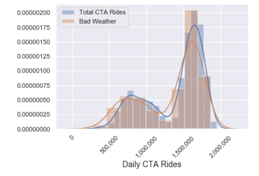
In other words, we found that bad weather has a statistically significant effect on CTA ridership, which is exactly what we had set out to prove. Abhishek congratulated us on a job well done, and I was happy to have drawn a tangible conclusion using real-world data. I was so inspired that I decided to download another data set from the Chicago Data Portal, this one about number of car crashes per day, and see if there was any significant correlation there.
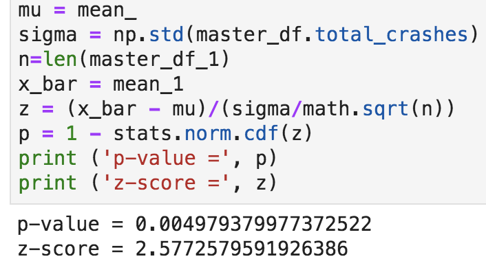
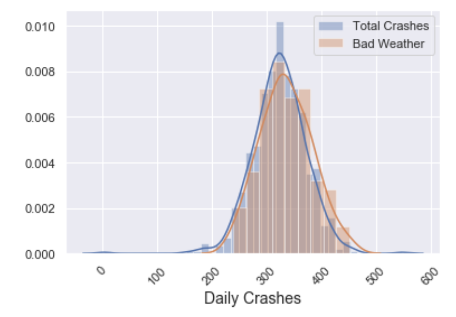
And it turns out there was. When I ran another test, this time using the null hypothesis that bad weather has no effect on car crashes, there once again was a statistically significant result, with a p-value less than 0.005:
I was feeling good about hypothesis testing.
Then we started learning linear regression. I had thought that linear regression and hypothesis testing were just two ways of doing the same thing. So with this in mind, I put the same data I had used in my car crash hypothesis test into an OLS regression, and this was the result:
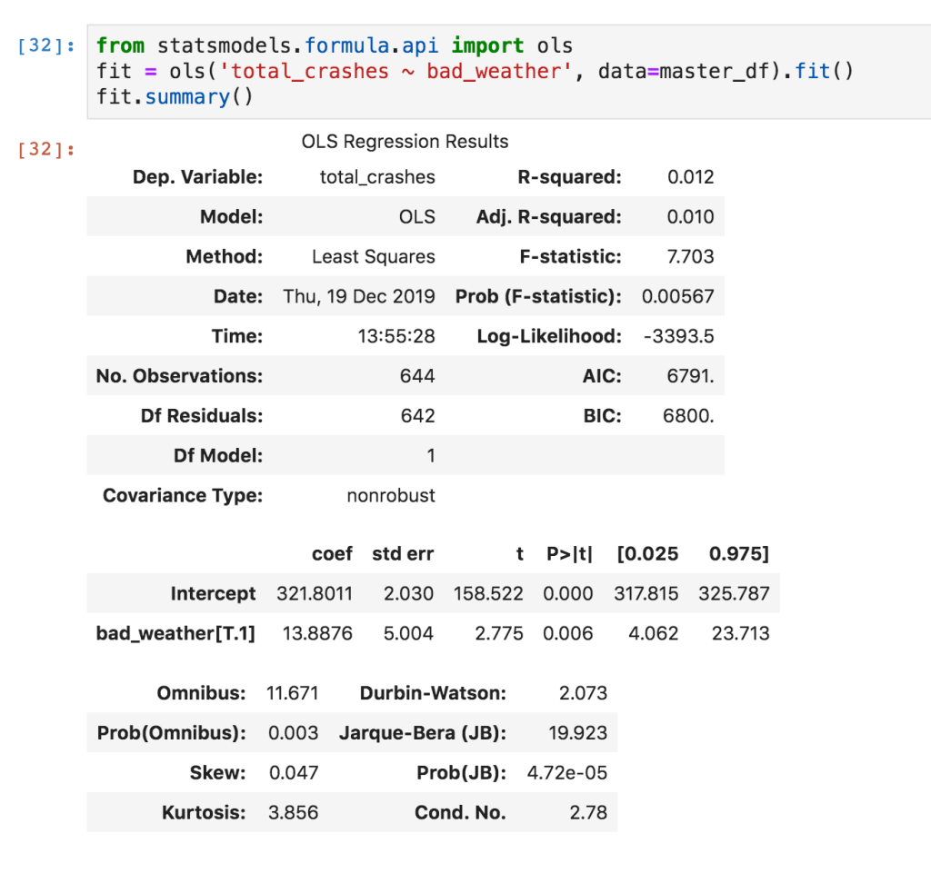
Once again, the p-value is significant, and I thought that this was the end of the story. However, Abhishek was walking by as I ran the test, and without even being asked a question, he pointed to the 0.012 R-squared value and simply said, “that’s a bad model”.
This confused me. It was the same data, and it had produced just as good of a p-value as the hypothesis test had. I didn’t realize that it was possible to have a low p-value and a low R-squared value at the same time.
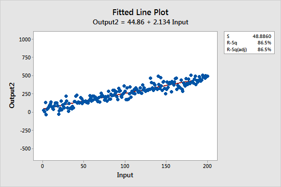
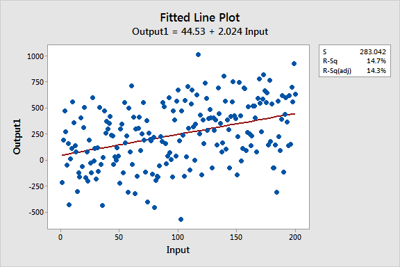
Fortunately, a quick Google search clearly illustrates this phenomenon of two distributions with similar coefficients and p-values, but with very different R-squared values:
The problem became much more obvious when I visualized the regression using Seaborn:
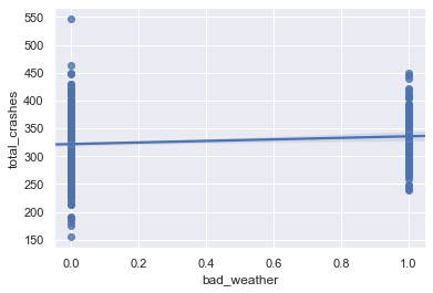
It turns out that a fundamental assumption of linear regression is that there is a linear relationship between the independent variable and the dependent variable. That is the data points should be as close as possible to the regression line, not on completely opposite ends of the graph as they are here.
That being said, the other three assumptions of linear regression didn’t seem to be violated at all:
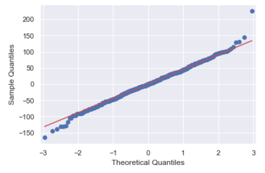
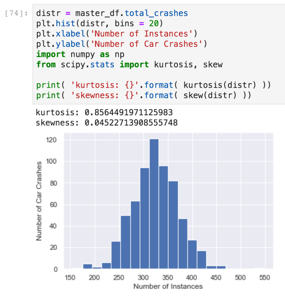
- 1) A qq-plot shows that the residuals are reasonably normally distributed. The entire distribution of car crash data is remarkably similar to a normal distribution, too, both in terms of skewness and in terms of kurtosis:
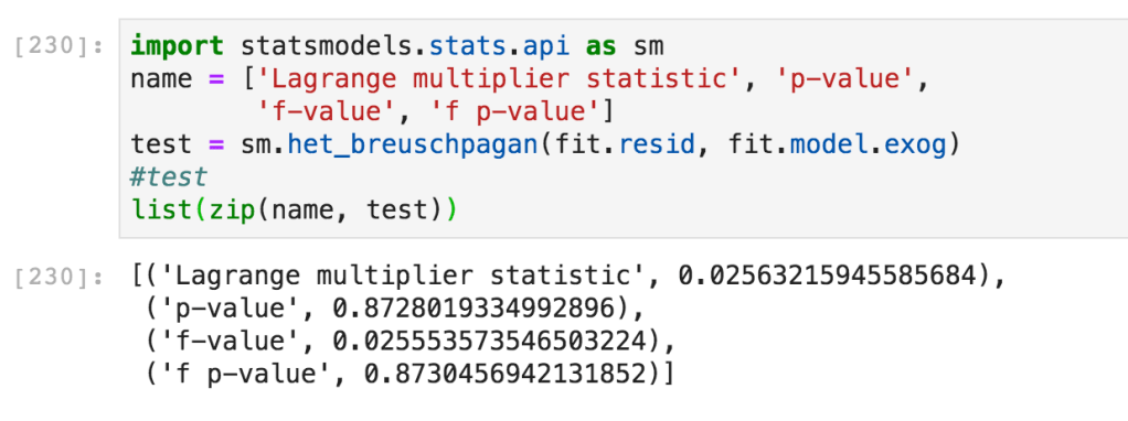
- 2) A Breusch Pagan test shows that we can’t reject the null hypothesis of homoscedasticity:
- 3) There is no multicollinearity, since there is only one independent variable.
Divide and Conquer
So regressing on a binary variable wasn’t going to work. But occurred to me that the daily “bad weather” categorical variable didn’t need to be binary. It had come from hourly weather data, and so it could be split into 25 different categories, each representing a number of hours in a day ranging from 0 to 24. I created a new ‘hourly bad weather’ variable, ran the regression again, and managed to raise the 0.012 R-squared value to a whopping 0.019.
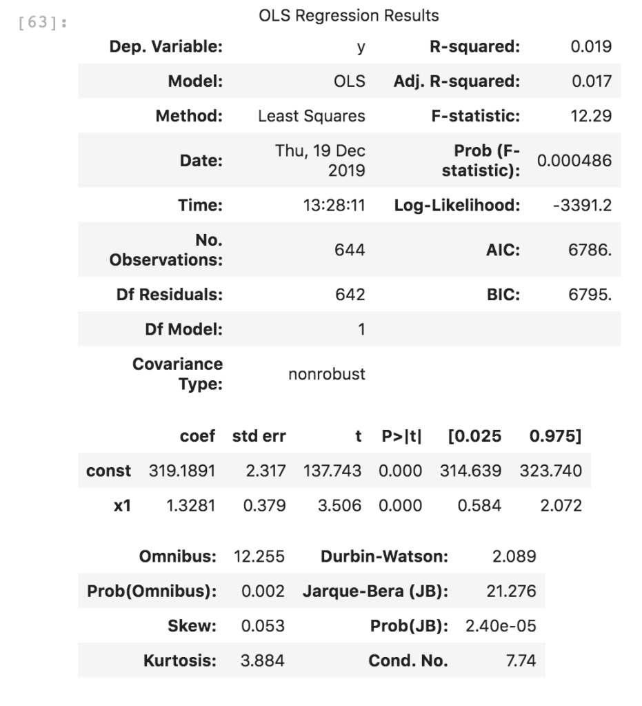
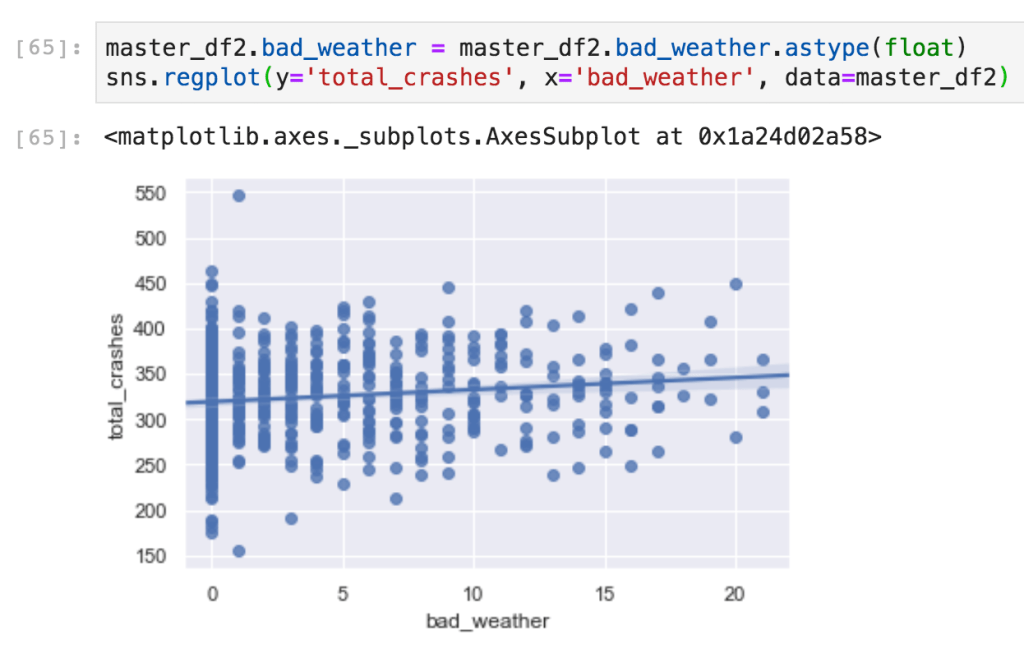
Long story short: bad weather, while having a significant effect on number of car crashes, accounts for less than 2% of the variation in number of crashes per day. If I wanted to gain any insight into the other 98%, I’d need to think of something else.
Time to Give Up?
I was ready to give up, but I had one last idea. Since I now had data for 22 unique “hours of bad weather in a day” values, I decided to take the average of each of them, and regress ‘total crashes’ on the result. The result was as follows:
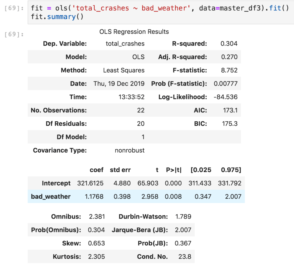
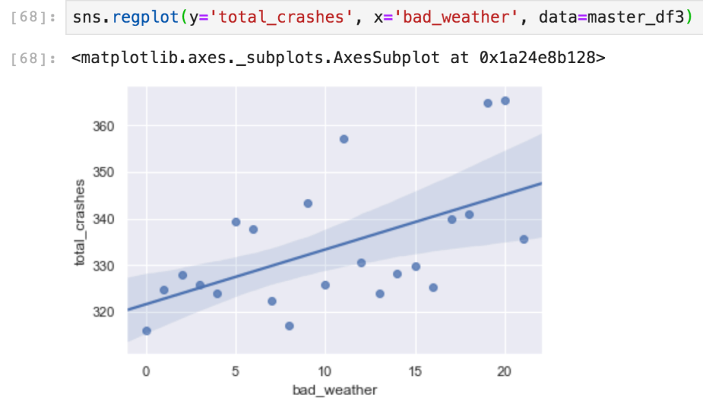
This yields an R-squared value of .304. It’s better, but at this point the model is pretty much useless. All it says is that, taking yearly aggregates, one extra hour of bad weather on a given day explains 30.4% of the 1.17-car increase in crashes.The other 69.6% is explained by something else.
But this is not surprising. There are so many factors involved in car crashes, it’s not surprising that my crude “bad weather” metric can only account for 30% of the variation in aggregate crash data. For example:
- My “bad weather” variable is not a consistent metric. “Rain” one hour isn’t identical to “rain” (or “snow”) another hour
- Car crashes are not completely independent events (e.g. multiple-car pileups)
- My “car crash” variable doesn’t take into account the severity of the crash
- Many crashes go unreported
Fun Facts
Since by now I had all of my formulas and models set up, I decided to run a few more tests, just to see if I could find anything interesting, or at least anything with an R-squared value higher than 0.019.
Crashes vs Temperature
There is an R-squared value of 0.039 (which at least is higher than 0.019) when regressing car crashes on near-freezing temperatures (temperatures between -5°C and 5°C). I thought this made sense. These are the temperatures that roads are beginning to freeze, are not salted, and drivers are not expecting the roads to be icy.
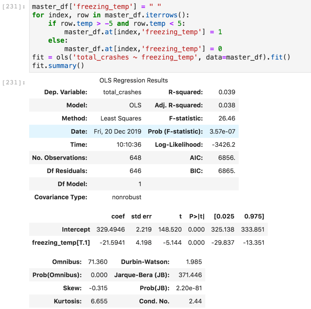
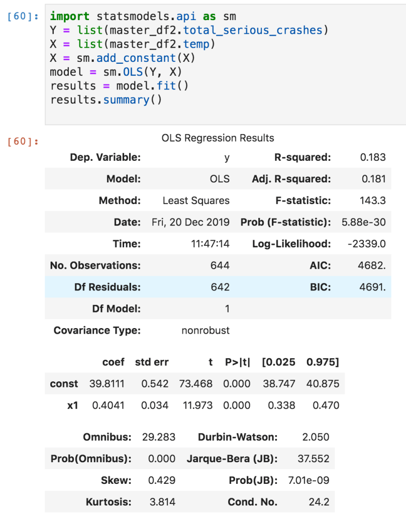
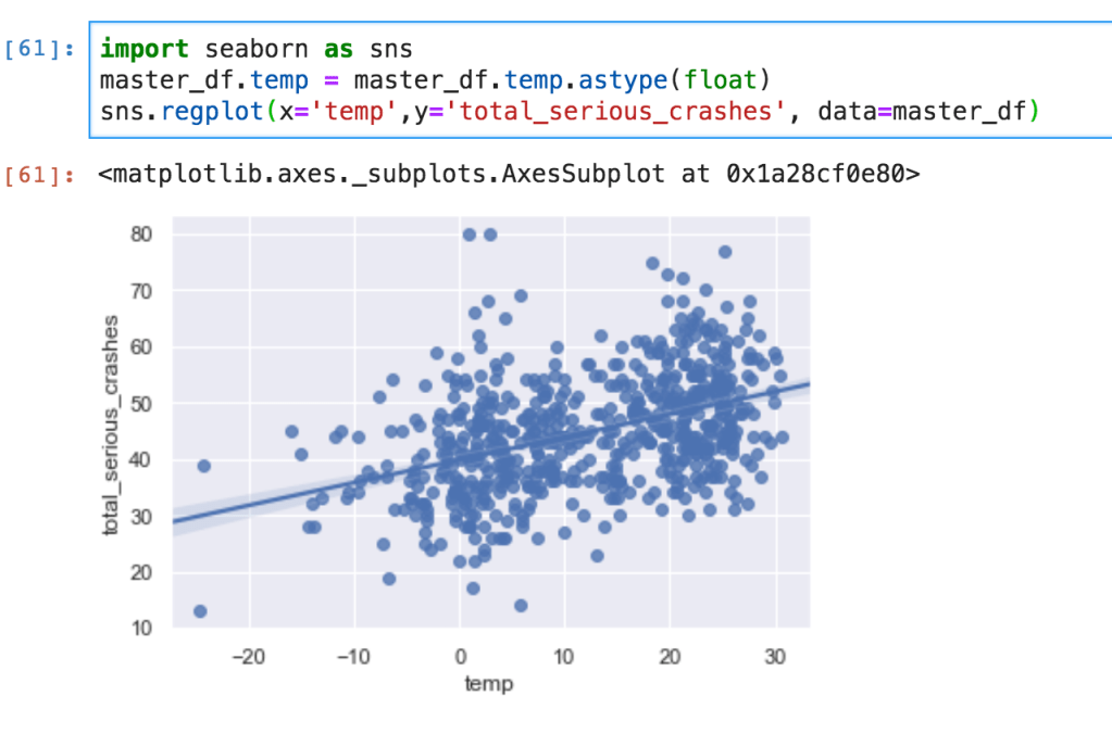
But if you look closely, the coefficient is negative, meaning that there are significantly fewer crashes on icy days, not more. One possibility for this could be that the crashes that occur on icy days are more serious. So I created a “serious crash” variable, which denoted crashes that resulted in at least one injury. This did not change the results, however. What did end up having more of a significant correlation was regressing number of serious crashes on temperature (in °C). This produced an R-squared value of 0.183:
Days of the Week
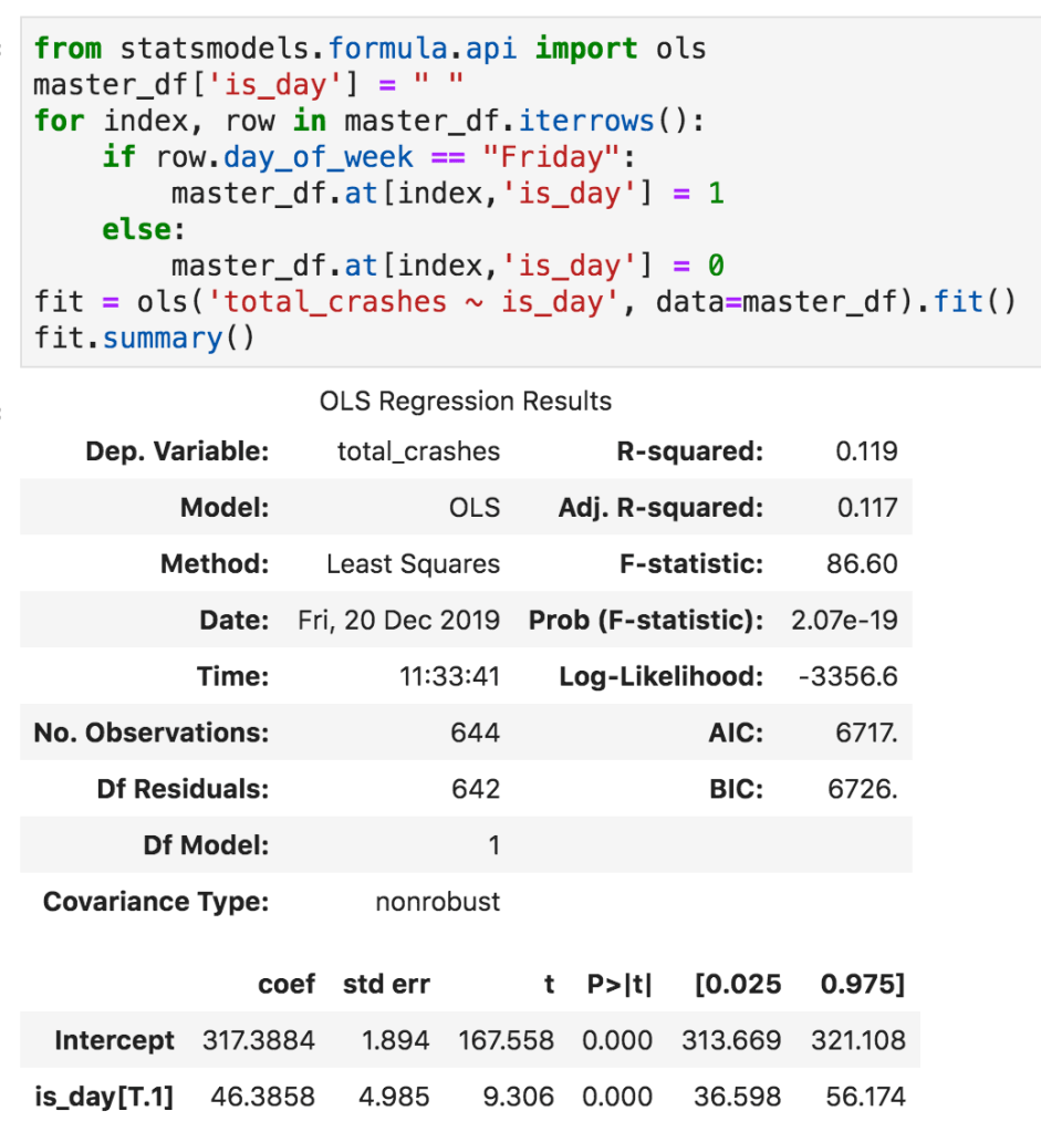
- There’s a 14.6% increase in car crashes on Friday:
- There’s a 16.6% decrease in car crashes on Sunday:
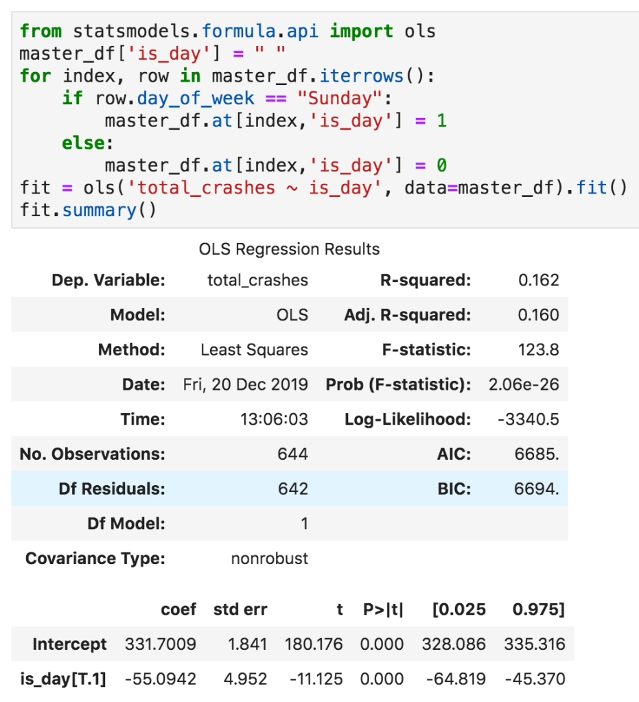
Both are highly statistically significant, but explain less than 17% of the variation in number of car crashes.
Conclusion
The purpose of hypothesis testing is to determine the validity of a particular claim. The purpose of linear regression, by contrast, is to determine the specific relationship between a dependent variable and one or more independent variables. Linear regression requires certain conditions to be met before any conclusions can be drawn. As such, it is not always appropriate to run a linear regression using data from a hypothesis test.
 Data, Data, Data